Line sim 3d
By Omar Essilfie-Quaye
Canvas is loading. Please wait.

Introduction - The Start of the Line
Line following is a trial that all roboticists have attempted to solve from the hobbyist to the professional. From one digital light sensor to hyper-spectral cameras there are many ways to make a robot follow a line. At the hobbyist level there are many competitions with a line following component. That can be following a line as fast as possible or using a line as a means of negotiating a complex environment. This extends to the industrial environment where lines are painted on factory floors to guide robots to drop off and pick up stock.
This simulation has been made to test some simple line following algorithms. As a hobbyist it can be quite difficult to know what is important in making a line following robot work. These parameters span the following: light sensor spacing, sensor size, robot speed, turning rate and algorithm. Playing with all of these variables at the same time can be quite hard, especially when some of them depend on hardware changes. This simulation provides a simple test bed to understand how the choices made can affect how well a robot follows a line.
This simulation is heavily inspired by RoboCup Junior Rescue Line . The rules for this competition are always updating and evolving to challenge the participants to come up with unique and creative solutions. The entire rule set is not implemented here please, visit the official website to learn about the current iteration of the rules.
Rules
- 1) The robot must follow the line at all times. If the robot loses the line it must start again from the beginning.
- 2) The robot must cross gaps without accidentally rejoining the line in the wrong position.
- 3) At "+" intersections the robot must go forwards.
- 4) At "T" intersections the robot must take the right most path.
- 5) When there is an immovable object on the line the robot must find a way around the object and back to the line within one tile.
- 6) The faster the robot completes the course the better the score.
One Sensor is All I Need
The most simplistic method to follow a line is with a single light sensor. This works in a very basic manner, if the light sensor is over the line turn right, otherwise turn left. This leads to a snake like back and forth motion. The behaviour that emerges from this is known as an edge follower, where the robot appears to be following the edge of the line rather than the centre of the line. There are a few variables in the algorithm that can be adjusted to slightly change the behaviour of the robot: the line detection threshold, the size of the light sensor and the turning speed.

Animation of a robot with one light sensor failing to cross a gap in the line that it is following.
All the changes and adjustments to the algorithm above can not account for a fundamental lack of information to base decisions on. This leads to the inability of the robot to cross gaps in the line. A robot with a single light sensor and a bearing sensor (be that a gyro or a compass) could reject turns over a white region that have a wide angle and back track. This could allow the robot to start a scanning routine to find the line on the other side of the gap.
Ok Maybe Two is Better
Twice the light sensors, twice the information. When you have two light sensors you can make more informed decisions about how to act in different scenarios. One method for following a line with two sensors is to use something known as a PID Control Loop. This takes a desired value and an error value and steers you towards the desired value based on how far away you are. The further away you are from the goal the harder you steer. For a line following robot you want both sensors to be on either side of the line and to read the same value. You can make the error the difference between the two light sensor readings. Just using the error value is called a P-controller, because your steering is proportional to the error.

Image of how two light sensors follow a line depending on which sensor has a darker reading.
A nice side effect of this system is that now when the robot is directly on the line it will go straight forwards, this is much quicker than constantly turning like with the one light sensor algorithm. It gets even better, now if the robot is not on a line it will still go forwards because the light sensor values are the same. This means that as long as the line preceding a gap is straight the robot with be able to cross the gap. If the line preceding the gap is at an angle, for example after a turn, the robot might miss the line on the other side. This is still an an improvement, but there is still not enough information to cross intersections in the correct direction.

Animation of a robot with two light sensors crossing multiple gaps.
Third Time is the Charm
The third central light sensor, is the key to negotiating intersections. In normal line following mode this sensor doesn't do much, the outer two sensors operate the same was as the two sensor algorithm. The third sensor provides an indication as to when the robot is over an intersection. When this is detected the robot can then complete a sweep and figure out which direction is the correct one to go in. The light sensor size and separation are crucial to this working as intended.

Animation of a robot with three light sensors negotiating line intersections.
The Simulation
This simulation is a model of what is happening in the real world. As per the common saying in the scientific community: " All models are wrong, but some are useful". This is particularly true for this line following simulation. The following section will delve into some of the trade-offs made to ensure that the simulation can run in real time whilst maintaining behaviours accurate to real line following robots.
The Line
Initially the model for the line was a pixel bitmap showing how much of a tile a line occupies. This was a simple model which produced results that were rather realistic. The real-time constraint for this project meant that manipulating images to take sensor readings was possibly too slow for the simple analog light sensor case. A series of points is used instead to represent the line. The Debug Static Tile mode will show how every single tile type is represented with individual points. Each tile is constructed with a minimum inter-point spacing to ensure that the line is well represented which is very important for curved lines.

Image showing the individual points that represent a line.
The Sensor
The main goal of a light sensor in this simulation is to provide a some means of measurement to identify where the line is. There are many means to do this using multiple types of sensor. In this simulation the aim will be to model a simple analog light sensor. This works by bouncing light off the surface below and seeing how much is returned. The greater the return the higher the voltage signal output by the sensor. This is affected by a series of parameters such as the intensity of the light, the height of the sensor above the surface and most importantly the material under the sensor. There are a number of assumptions that are made for this simulation.

Image showing that the light sensor only looks at the closest line point.
Assumptions
- 1) There are no external light sources and the onboard light source is not fluctuating as is common when lights are powered with unstable power supplies.
- 2) The height of the light sensor above the ground is constant. This means that the area of the circle remains constant all the time. This is generally quite difficult to achieve on a robot. Even with active suspension maintaining a perfectly stable height is unlikely.
- 3) The material of the background perfectly reflects light in a uniform manner across all the tiles in the room. This will return the maximum of 1.0f when the light sensor is fully over the background.
- 4) The material of both the line perfectly absorbs light in a uniform manner across all the tiles in the room. This will return the maximum of 0.0f when the light sensor is fully over the black line.

Exaggerated line point spacing showing how lines behave.

Condensed line point spacing still showing small gaps at the edges.

Graph showing how the light sensor value changes due to the line point model. This effect is reduced at the centre of the line.
The graph on the right hand side shown above is an example of how these spikes in sensor value could appear. This graph is obtained by taking a simple analog sensor and moving it at uniform speed along the edge of a line. The expected value of the light sensor reading is 0.5f. The individual lines shown are for light sensors with larger and large radius. This reduces the effect of the gaps between the line points as they take up less area in the light sensors field of view. Similarly if the inter point distance is reduced the errors will also be smaller.
Whilst these errors are unavoidable they can be quantified more precisely to understand if they are acceptable. For example looking at the maximum, minimum and average of the light sensor error for all the positions recorded above can provide an understanding of the overall performance for a given set of parameters. This can be seen in the following graph. For example if the light sensor radius and the line point separation are the same then there is a less than 5% mean error.


